The authors: Grigoriy Belyavskiy, Valentina Misyura, Evgeny Puchkov

Introduction

At the prediction for the time series there are problems of the noise, the non-stationarity, and we don’t have enough information to choose the financial market model. In this situation, the usage of an artificial neural network is justified. It allows obtaining non-linear and non-stationary models using the training algorithm and window method [1].

Consider the time series as a realization of a stochastic process $\{X_\tau, 0 \le \tau \le t \}$. The object of research is a discrete analogue of the equation, $dX_\tau = \alpha (t, \{ X_\tau, 0 \le \tau \le t \})dt + \beta (t, \{ X_\tau, 0 \le \tau \le t \})dW_t$ , where coefficients are time and trajectory functional of a stochastic process.

One approach of solving the time series prediction problem uses wavelet transforms and artificial neural networks (ANN), which are well described in the scientific publications [2, 3, 4, 5, 6]. In some cases, wavelet transformation is used for initial data transformation, which is submitted to the network as training examples. In other cases, network signals are transformed with wavelet-basis usage.

In this work possibility of the time series prediction using neural network model based on a wavelet-core is investigated. The problem of a confidential interval prediction is considered. The prediction of a confidential interval is more effective than the point prediction for decision making. One more feature is using the order statistics in addition to values of the time series in the training sample. The basic complexity of a problem consisted in the training algorithm. The hybrid algorithm has been used. It combines the gradient method with the genetic algorithm. The evolutionary computations are used to evaluate the gradient. It has allowed to avoid difficult computations of the gradient during iterations.

Prediction Methodology

Problem Statement

Consider the stochastic process model:

where $\varphi$ is function equal to zero outside some finite interval $[0, A]$ and belongs to space $L_2 [0,A]$, $\varepsilon$ - sequence of independent, standard normal random variables. Model (1) related to conditionally Gaussian models with conditional distribution law $Law(X_n/F_{n-1}) = N(a_0 + \Sigma_{i=1}^{p}a_i X_{n-i}, \varphi (b_0 + \Sigma_{i=1}^{q}b_i X_{n-i}^{2}))$ , where $F_i = \sigma(\varepsilon_{1}, ..., \varepsilon_{i})$ , that allows to find the joint density $p(x_1, x_2, ..., x_n) = (2\pi)^{-n/2} \Pi_{k=1}^{n} \varphi (b_0 + \Sigma_{i=1}^{q} b_i x_{k-i}^{2})exp(-\frac{1}{2} \Sigma_{k=1}^{n} \frac{(x_k - a_0 - \Sigma_{i=1}^{p} b_i x_{k-i})^{2}}{\varphi(b_0 + \Sigma_{i=1}^{q} b_i x_{k-i}^{2})})$ for fixed $x_{1-l}, ..., x_0$ , where $l = max\{ p,q\}$. In the particular case, when $\varphi (x) = \sqrt{x}$ over interval $[0, A]$ , Equation (1) is $AR(p)/ARCH(q)$ - equation [7].

There is no second component of the model – stochastic volatility in the evaluation of the conditional expectation $\underline{X}_n = E(X_n / F_{n-1}) = a_0 + \Sigma_{i=1}^{p} a_i X_{n-i}$. This is the main disadvantage of the one-step prediction problem. The prediction of a confidential interval is more effective.

Assume that 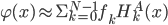$\varphi (x) \approx \Sigma_{k=0}^{N-1} f_k H_k^{A} (x)$ was calculated with a high degree of accuracy, where $H_k^{A} (x)$ - wavelet - basis on the interval $[0, A]$ for example, Haar basis [8], built on the basis of maternal functions:

Then the confidence interval prediction with a fixed confidence probability $1-\alpha$ equal to

when $X_n^{+}, X_n^{-}$ – the upper and lower predictive estimates of the stochastic process, respectively, the parameter $k$ - a solution of the equation $\Phi (x) = 1-\frac{\alpha}{2}$, where $\Phi (x)$ - a function of the standard normal distribution.

Architecture of Wavelet Neural Network

The research about neural network representation of nonlinear stochastic time series models are found in literature about neural network design and applications [9, 10, 11, 12, 13]. The complexity of this types of models is overcome by a specially selected ANN architecture and evaluating the weight coefficients. An important fact is that the weights included in the neural network model linearly. The architecture of a ANN  according to equations (3) is illustrated in Figure 1.

A major advantage of the proposed solution is wavelet package included in ANN. It has allowed don’t fix the function $\varphi$ and has made a ANN is sufficiently universal.  The determination of weights is achieved by solving the problem of training.

The problem of ANN training consists of calculating the parameters $\{a\}, \{b\}$ and $\{f\}$ using training data set $V = \{ 1, X_{n-p}, ..., X_{n-1}; 1, X_{n-q}^{2}, ..., X_{n-1}^{2}; X_{\alpha / 2}^{-}, X_{\alpha / 2}^{+}\}$, where $X_{\alpha / 2}^{-}, X_{\alpha / 2}^{+}$ - a output values of the ANN (a lower and upper $\alpha / 2$ quartiles). As noted in the literature, see, eg, [14], sample quantiles have a wide range of quality properties.

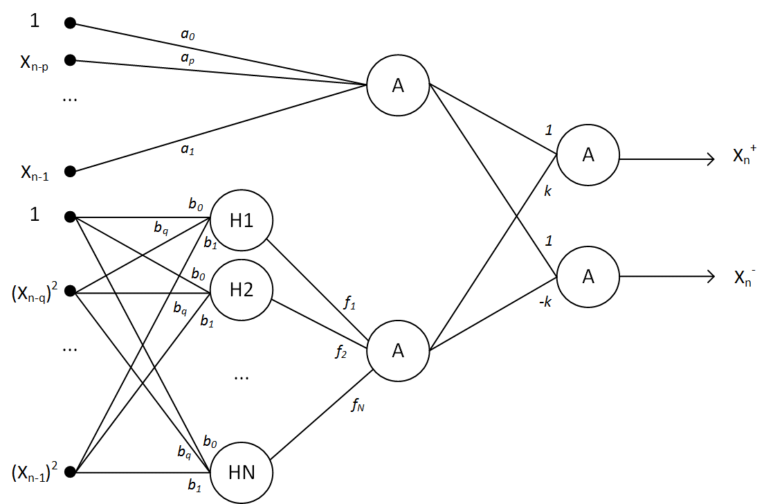
Fig. 1. Architecture of ANN based on wavelet-core

Training Algorithm

The proposed algorithm uses the idea of the adaptive algorithm described in  [15 ]. The ANN is trained on  training set $\{V^{(k)} \}_{k \ge 1}$.The quality criterion of training is the mean square error:

Let the parameter space $R^m$. The dimension of space 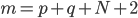$m = p+q+N+2$ coincides with the number of adjustable parameters, including wavelet decomposition. Accordingly, the quality criterion (4) will be considered as a function of $m$ variable - $F (x_1, x_2, ..., x_m)$. The training algorithm was defined by the recurrent relation:

where $g_0 = \bigtriangledown F(P^0)$. The gradient calculation $\bigtriangledown F$ is a computationally challenging task for the considered ANN architecture. The backpropagation algorithm is one way to solve it. Another way to do it is to replace the gradient with some analogue, which is calculated more easily. For example, the partial derivative of one of the variables can be replaced by a corresponding difference: $\frac{dF(P)}{dx_i} \approx \frac{F(P+\varepsilon e_i) - F(P)}{\varepsilon}$.

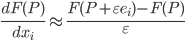Consider the hyperplane $z-(A,P)=0$, that passes through the points $(P, F(P)), (P + \varepsilon e_1, F(P+varepsilon e_1)), (P + \varepsilon e_2, F(P+varepsilon e_2)), ..., (P + \varepsilon e_i, F(P+varepsilon e_i))$, where the $i$-th is vector coordinate 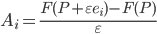$A$, $A_i = \frac{F(P+\varepsilon e_i) - F(P)}{\varepsilon}$. If we generalize this fact then $z = F(\overline{P})$ should be approximated in a neighbourhood of a point $P$ using $z = (A, P)$ for the gradient calculation and $\bigtriangledown F(P) \approx A$. $\varepsilon$ - neighbourhood of a point $P$ is the hypercube 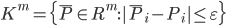$K^m = \{ \overline{P} \in R^m : | \overline{P}_i - P_i| \le \varepsilon\}$. The largest approximation error occurs at the vertices of a hypercube: $P^{\delta} = P+\varepsilon \Sigma_{i=1}^{m} (-1)^{\delta_i} e_i$, where $\delta_i \in \{0,1\}$. Therefore, the calculation of the vector $A$ is necessary to consider the system of linear equations for all the vertices of a hypercube $(A, P^{\delta}) = F(P^{\delta})$. Using the method of least squares we get a system of linear equations:

where $i$-th row of the matrix $H - Row (H)_i = \{(-1)^{\delta_k (i)}\}, \delta_k (i) - k$-th digit binary code of number $i$, $i$-th vector coordinate $Z - Z_i = F(P^{\delta (i)})$. The dimension of the system coincides with the dimension of the parameter space. The matrix size $H - (2^m, m)$, therefore, the calculation of the system (6) may require significant computational cost.

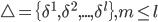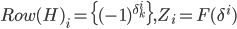Consider the compromise version of calculation. We will select the set of vertices $\bigtriangleup = \{ \delta^1, \delta^2, ..., \delta^l\}, m \le l$, where $l$ significantly less than $2^m$, and $Row(H)_i = \{(-1)^{\delta_{k}^{i}}\}, Z_i = F (\delta^i)$. The vertices in the set  are selected by using a genetic algorithm [16].

The algorithm of hypercube vertices selection:

1. Generate a random initial population of $l$ chromosomes – binary sets. Calculate fitness function minimum $F(P^{\delta^i})$ for each set $\delta^i$. (The less $F(P^{\delta^i})$ the healthier chromosome).
2. Select $r$ pairs for crossing with probabilities inversely proportional to the fitness $c/F(P^{\delta^i})$. The number $r \le l/2$.
3. For each gene it’s been randomly determined with adjusted probability whether it will be crossed or not. If yes, there is a data exchange between parents. Thus, each pair produces 2 descendants. Calculate the fitness function for the descendants.
4. Generate a new population of $l$ chromosomes using natural selection.

The algorithm will works as long as the population is stabilized. The set of hypercube vertices for a gradient calculation is constructed.

Experiments

The results of the method verification for interval prediction of stochastic processes to model data presented in [17]. Further the results of experiments on real data is presented. RTS index and S&P 500 for analysis and testing of the described method were selected. Daily index values from 11.08.2015 to 02.02.2016 for experiments was used. Predictions for sample data volume 121 observation were performed.

Data Preparation

The method of a sliding "window" with a fixed size w for the training sets in time series prediction problem was used. The univariate time series $X_n$ using shear procedure into two samples $X_n^{+}, X_n^{-}$ was converted. These are upper and lower one-step predictive estimate of a stochastic process, respectively.

The lower and upper bounds of the confidence interval sample median as the target variables for training the ANN was used. The intervals using the values of the current "window" with a fixed confidence probability were found. The median is statistically stable estimation if data in the sample will stand out or differ markedly from each other [18]. The visualization of the obtained training sets are illustrated in Figure 2 and Figure 3.

Fig. 2. RTS index training data set: w=9, α=0,2

Fig. 3. S&P 500 training data set: w=9, α=0,2

Results

A original data set into two samples was splitted. The first of which is used to train ANN (100 values of training data set) and the second is used to validate the model (20 values of test data set). The window (w) size equal 9 for sample quantiles was used. Wavelet-basis contained 8 functions. The prediction results for training and test sets using the ANN is illustrated in Figures 4-7.

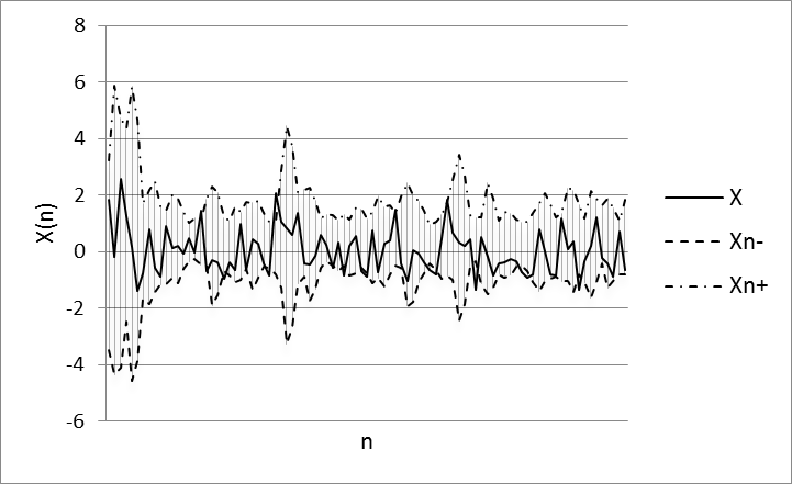
Fig. 4. Experiment results using RTS training data set.
Parameters of model: w=9, α=0,2, N=8

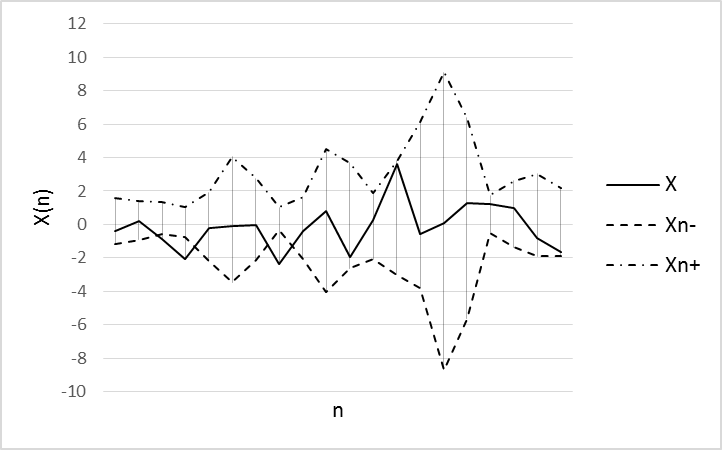
Fig.5. Experiment results using RTS test data set.
Parameters of model: w=9, α=0,2, N=8

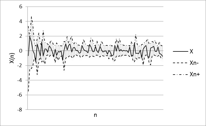
Fig. 6. Experiment results using S&P 500 training data set.
Parameters of model: w=9, α=0,2, N=8

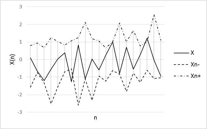
Fig.7. Experiment results using S&P 500 test data set.
Parameters of model: w=9, α=0,2, N=8

Conclusion

ANN based on wavelet-core is a fairly universal tool for time series prediction using conditionally Gaussian models. Function $\varphi$ determines substantial non-linearity of the model. The greatest effect is achieved when the function $\varphi$ into a rapidly convergent series in the wavelet basis is decomposed. The basic complexity of a problem consisted in the training algorithm. The hybrid algorithm has been used. It combines the gradient method with the genetic algorithm. The prediction results show expediency and efficiency of the proposed method.

References

1. Li, W. Ma, Applications of artificial neural networks in financial economics: a survey, Proceedings of the 2010 International Symposium on Computational Intelligence and Design, IEEE Computer Society. 01 (2010), 211–214.
2. J. Hsieh, H.F. Hsiao, W.C. Yeh, Forecasting stock markets using wavelet transforms and recurrent neural networks: an integrated system based on artificial bee colony algorithm, Appl. Soft Comput. 11 (2011), 2510–2525.
3. Lahmiri, Wavelet low- and high-frequency components as features for predicting stock prices with backpropagation neural networks, Journal of King Saud University - Computer and Information Sciences. 26 (2) (2014), 218-227.
4. Alexandridis, A. Zapranis, Wavelet neural networks: A practical guide, Neural Networks. 42 (2013), 1-27.
5. Zhao, G. Wang, Application of Chaotic Particle Swarm Optimization in Wavelet Neural Network, TELKOMNIKA (Telecommunication Computing Electronics and Control). 12 (4) (2014), 997.
6. Chen, B. Yang, J. Dong,Time-series prediction using a local linear wavelet neural network, Neurocomputing. 69, (4-6) (2006), 449–465.
7. N. Shiryaev, Osnovy stokhasticheskoy finansovoy matematiki. Fakty. Modeli, FAZIS, Moscow, 1998.
8. A. Zalmanzon, Preobrazovaniya Fur'e, Uolsha, Khaara i ikh primenenie v upravlenii, svyazi i drugikh oblastyakh, Nauka. Gl. red. Fiz.-mat. Lit., Moscow, 1989.
9. Dente, R. Mendes, Characteristic functions and process identification by neural networks. arXiv:physics/9712035v1 [Physics data-an], 17 Dec. (1997), 11.
10. Beer, P. Spauos, Neural network based Monte Carlo simulation of random processesm. ICOSSAR, G Augusti, G. Shueller, MCiampoli as ed., Millpress, Roterdam, 2005.
11. Balasubramaniam, P. Vembarasan, R. Rakkiyappan, Delay-dependent robust exponential state estimation of Markovian jumping fuzzy Hopfield neural networks with mixed random time-varying delays, Commun Nonlinear Sci Numer Simulat. 16, (2011), 2109–2129.
12. Leen, R. Friel, D. Nielsen, Approximating distributions in stochastic learning, Neural Networks 32 (2012), 219–228.
13. Han, L. Wang, J. Qiao, Efficient self-organizing multilayer neural network for nonlinear system modeling, Neural Networks. 43 (2013), 22–32.
14. Veroyatnost' i matematicheskaya statistika: Entsiklopediya, Pod red. Yu.V.Prokhorova , Bol'shaya rossiyskaya entsiklopediya, Moskva, 2003.
15. I. Belyavskiy, V.B. Lila, E.V. Puchkov, Algoritm i programmnaya realizatsiya gibridnogo metoda obucheniya iskusstvennykh neyronnykh setey, Programmnye produkty i sistemy. 4 (2012), 96-101.
16. N.H. Siddique, M.O. Tokhi, Training neural networks: backpropagation vs. genetic algorithms, Neural Networks 4 (2001), 2673 – 2678.
17. I. Belyavskiy, I.V. Misyura, Neyrosetevoy predskazatel' s veyvlet-yadrom, Izvestiya vysov uchebnykh zavedeniy, Severo-Kavkazskiy region, Estestvennye nauki. 3 (2014), 11 – 13.
18. A. David, H. N. Nagaraja, Order Statistics, 3rd Edition. Wiley, New York, 2003.